45 how to add labels to charts in excel

40 how to add different data labels in excel How to Add Data Labels to an Excel 2010 Chart - dummies If you don't want the data label to be the series value, choose a different option from the Label Options area. You can change the labels to show the Series Name, the Category Name, or the Value. Select Number in the left pane, and then choose a number style for the data labels. 42 how to turn on data labels in excel Adding Data Labels to a Chart Using VBA Loops - Wise Owl To do this, add the following line to your code: 'make sure data labels are turned on FilmDataSeries.HasDataLabels = True This simple bit of code uses the variable we set earlier to turn on the data labels for the chart.

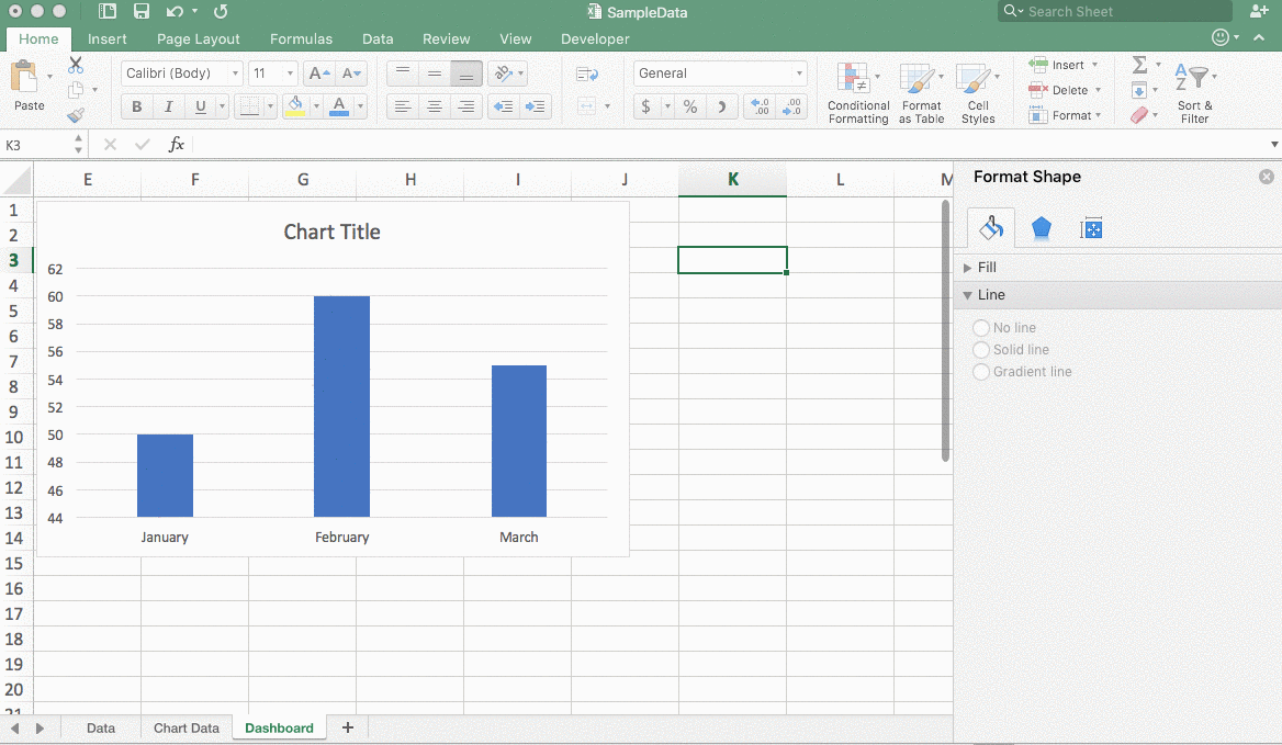
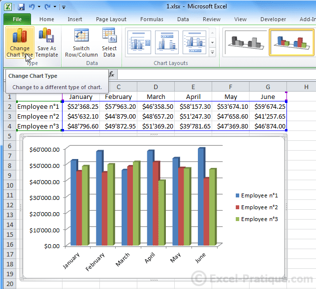
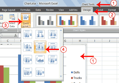
Creating and Modifying Charts - Using Microsoft Excel ... In all cases, you have to select the chart first to access Chart Tools. To add any labels (for example, the title or axes), under the Design ribbon, click Add Chart Element in the Chart Layouts group and select the desired label. To change the chart type, data, or location, use the Chart Tools Design ribbon.

How to add labels to charts in excel

Steps on How to Add a Legend in Excel (With Tips and FAQs ... 1. First method. Below are the procedures to follow when employing the first method to add a legend in Excel: Click on the chart. The first step is to click on the chart to generate 3 bars at the top-right section of the chart. The three buttons help you modify the chart. Click on the "Chart Elements" button. Use defined names to automatically update a chart range ... On the Insert menu, click Chart to start the Chart Wizard. Click a chart type, and then click Next. Click the Series tab. In the Series list, click Sales. In the Category (X) axis labels box, replace the cell reference with the defined name Date. For example, the formula might be similar to the following: =Sheet1!Date How to Create a Line Chart in Microsoft Excel Select the data you want to display in the chart and go to the Insert tab. Click the Insert Line or Area Chart drop-down arrow. Choose the type of line chart you want to use. On Windows, you can...

How to add labels to charts in excel. How to Add Labels to Scatterplot Points in Excel - Statology Step 3: Add Labels to Points. Next, click anywhere on the chart until a green plus (+) sign appears in the top right corner. Then click Data Labels, then click More Options…. In the Format Data Labels window that appears on the right of the screen, uncheck the box next to Y Value and check the box next to Value From Cells. Excel: How to Create a Bubble Chart with Labels - Statology To add labels to the bubble chart, click anywhere on the chart and then click the green plus "+" sign in the top right corner. Then click the arrow next to Data Labels and then click More Options in the dropdown menu: In the panel that appears on the right side of the screen, check the box next to Value From Cells within the Label Options ... How to Apply a Filter to a Chart in Microsoft Excel Select the chart and you'll see buttons display to the right. Click the Chart Filters button (funnel icon). When the filter box opens, select the Values tab at the top. You can then expand and filter by Series, Categories, or both. Simply check the options you want to view on the chart, then click "Apply." Advertisement How to add legend title in Excel chart - Data Cornering Add legend title in Excel chart. Select an Excel chart to add a text box. This is important to bound chart and textbox together. Otherwise, the Excel chart and text box move separately. Go to the Insert tab, and on the right side will be a text box. Selec and draw it over the place where you want it in the chart.

Make better Excel Charts by adding graphics or pictures ... You can hold down the CTRL key as you're adjusting to keep the center of the image in the same place. You can hold down the Shift Key as you're adjusting to maintain the picture's proportions. You can hold down CTRL + Shift key at the same time to do both. Repeat for any other images you'd like to add. Only add images to a fixed chart. Bar Chart in Excel - Types, Insertion, Formatting - Excel ... To add Data Labels to the chart, perform the following steps:- Click on the Chart and go to the + icon at the top right corner of the chart. Mark the Data Labels from there After that, select the Horizontal Axis and press the delete key to delete the horizontal axis scale. This is how the chart looks once finished. How to Add Axis Titles in a Microsoft Excel Chart Select your chart and then head to the Chart Design tab that displays. Click the Add Chart Element drop-down arrow and move your cursor to Axis Titles. In the pop-out menu, select "Primary Horizontal," "Primary Vertical," or both. If you're using Excel on Windows, you can also use the Chart Elements icon on the right of the chart. How to Find, Highlight, and Label a Data Point in Excel ... Following are the steps: Step 1: Add a new table with three new columns in it.This table helps you input the cell you want to highlight. Step 2: Enter the Student name you want to highlight in your scatter chart.For example, Arushi.Now, our task is to find the Hours studied and Marks Obtained from the student name entered.You can use the VLOOKUP function for this.

Modifying Axis Scale Labels (Microsoft Excel) In the Category list, choose Custom. In the Type box, enter a zero followed by a comma. Click OK. Only the thousands portion of the values in the axis should be displayed. You can then add another label, as desired, that indicates the values are expressed in thousands. How to create pill charts in Excel - spreadsheetweb.com The most important addition is the Data Labels if you want to express actual values on the chart. Because of the helper columns, the visual cannot provide the precise values and differences between bars. Adding Data Labels removes this issue. Select the actual data parts on the chart and use the Chart Elements button to add the Data Labels. excel - Formatting Data Labels on a Chart - Stack Overflow sub charttest () activesheet.chartobjects ("chart 6").activate z = 1 with activechart if .charttype = xlline then i = .seriescollection (1).points.count activechart.fullseriescollection (1).datalabels.select for pts = 1 to i activechart.fullseriescollection (1).points (pts).hasdatalabel = true ' make sure all points are visible data … How to Create a Run Chart in Excel (2021 Guide) | 2 Free ... Download this Excel run chart template with dynamic data labels. Note: Since your median is going to be different, you need to adapt the custom number formatting accordingly ( Format Data Labels > Label Options > Number > Format Code > In the " Format Code " field, replace " 80 " with your median value as shown below).

How to Create an Excel Dashboard in 7 Steps | GoSkills

How to Create a Population Pyramid Chart in Excel - Sheetaki Select the axis label element to pull up the Format Axis panel. Under the Labels section, select the Low option. In the Format Data Series panel, change the Series Overlap to 100% and Gap Width to 0%. You can also add a solid line as a border for each bar in the population pyramid chart.

Excel Course: Inserting Graphs

How to Create a Waterfall Chart in Excel - SpreadsheetDaddy By default, most charts will have some form of data label automatically applied, but you can also add your own custom labels if needed. Let's see how to do it! 1. Click on your chart. 2. Navigate to the Design tab. 3. Choose Add Chart Element. 4. Click Data Labels. 5.

Format Number Options for Chart Data Labels in Excel 2011 for Mac

Shapes.AddLabel method (Excel) | Microsoft Docs The text orientation within the label. Left: Required: Single: The position (in points) of the upper-left corner of the label relative to the upper-left corner of the document. Top: Required: Single: The position (in points) of the upper-left corner of the label relative to the top of the document. Width: Required: Single: The width of the ...

Where Do I Put The Label? In Excel – Excel-Bytes

Add or remove data labels in a chart - Microsoft Support

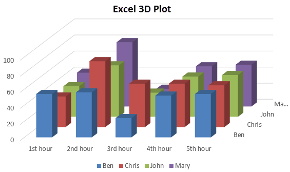
3D Plot in Excel | How to Plot 3D Graphs in Excel?

How to Create Multi-Category Charts in Excel? - GeeksforGeeks Step 1: Insert the data into the cells in Excel. Now select all the data by dragging and then go to "Insert" and select "Insert Column or Bar Chart". A pop-down menu having 2-D and 3-D bars will occur and select "vertical bar" from it. Select the cell -> Insert -> Chart Groups -> 2-D Column Bar Chart Insertion Multi-Category Chart

Excel Charts

How to Create Charts in Excel: Types & Step by Step Examples Below are the steps to create chart in MS Excel: Open Excel. Enter the data from the sample data table above. Your workbook should now look as follows. To get the desired chart you have to follow the following steps. Select the data you want to represent in graph. Click on INSERT tab from the ribbon. Click on the Column chart drop down button.

Share :